Technological set and its properties. The concept of a production system and a production process. Technological process and technological set. Properties of production sets
Ministry of Education and Science of the Russian Federation
Yaroslav the Wise Novgorod State University
Discipline abstract:
Management
Performed by a student from group 6061 zo
Makarova S.V.
Received by Suchkov A.V.
Velikiy Novgorod
1. PRODUCTION PROCESS AND ITS ELEMENTS.
The basis of the production and economic activity of the enterprise is the production process, which is a set of interrelated labor processes and natural processes aimed at the manufacture of certain types of products.
The organization of the production process consists in uniting people, tools and objects of labor into a single process for the production of material goods, as well as in ensuring a rational combination in space and time of the main, auxiliary and service processes.
Production processes at enterprises are detailed by content (process, stage, operation, element) and place of implementation (enterprise, redistribution, workshop, department, site, unit).
The multitude of production processes that take place in an enterprise is a cumulative production process. The production process of each individual product of the enterprise is called private production process... In turn, in a private production process, partial production processes can be distinguished as complete and technologically separate elements of a private production process, which are not the primary elements of the production process (as a rule, it is carried out by workers of different specialties using equipment for various purposes).
The primary element of the production process should be considered technological operation- a technologically homogeneous part of the production process carried out at one workplace. Technologically isolated partial processes are stages of the production process.
Partial production processes can be classified according to several criteria:
By intended purpose;
The nature of the flow in time;
The way of influencing the subject of labor;
The nature of the labor employed.
Processes are distinguished according to their intended purpose main, auxiliary and service.
The main production processes - the processes of converting raw materials and materials into finished products, which are the main, profile
products for this enterprise. These processes are determined by the manufacturing technology of this type of product (preparation of raw materials, chemical synthesis, mixing of raw materials, packaging and packaging of products).
Subsidiary manufacturing processes are aimed at the manufacture of products or the provision of services to ensure the normal course of the main production processes. Such production processes have their own objects of labor, different from the objects of labor of the main production processes. As a rule, they are carried out in parallel with the main production processes (repair, container, tool facilities).
Serving production processes ensure the creation of normal conditions for the flow of main and auxiliary production processes. They do not have their own subject of labor and proceed, as a rule, sequentially with the main and auxiliary processes, interspersed with them (transportation of raw materials and finished products, their storage, quality control).
The main production processes in the main shops (sections) of the enterprise and form its main production. Auxiliary and service production processes, respectively, in auxiliary and service shops - form an auxiliary farm.
The different role of production processes in the total production process determines the differences in the mechanisms of management of various types of production units. At the same time, the classification of partial production processes according to their intended purpose can be carried out only in relation to a specific private process.
The combination of the main, auxiliary, service and other processes in a certain sequence forms the structure of the production process.
The main production process represents the process and production of main products, which includes natural processes, technological and work processes, as well as interoperative bedding.
A natural process is a process that leads to a change in the properties and composition of the object of labor, but takes place without human participation (for example, in the manufacture of certain types of chemical products).
Natural production processes can be considered as necessary technological breaks between operations (cooling, drying, aging, etc.)
Technological a process is a set of processes as a result of which all the necessary changes occur in the subject of labor, that is, it turns into a finished product.
Ancillary operations facilitate the performance of basic operations (transportation, control, product sorting, etc.).
Work process - the totality of all work processes (main and auxiliary operations).
The structure of the production process changes under the influence of the technology of the equipment used, the division of labor, the organization of production, etc.
Interoperative bed - breaks provided by the technological process.
By the nature of the flow in time, there are continuous and periodic production processes. In continuous processes, there are no interruptions in the production process. Production maintenance operations are performed simultaneously or in parallel with the main operations. In periodic processes, the execution of the main and service operations occurs sequentially, due to which the main production process is interrupted in time.
According to the method of influence on the subject of labor, they distinguish mechanical, physical, chemical, biological and other types of production processes.
By the nature of the labor used, production processes are classified into automated, mechanized and manual.
The principles of the organization of the production process are the starting points, on the basis of which the construction, functioning and development of the production process are carried out.
There are the following principles for organizing the production process:
differentiation - the division of the production process into separate parts (processes, operations, stages) and their assignment to the corresponding divisions of the enterprise;
combining - combining all or part of diverse processes for the manufacture of certain types of products within one site, workshop or production;
concentration - the concentration of certain production operations for the manufacture of technologically homogeneous products or the performance of functionally homogeneous work at individual workplaces, areas, in workshops or production facilities of an enterprise;
specialization - assigning a strictly limited range of works, operations, parts and products to each workplace and each division;
universalization - the manufacture of parts and products of a wide range or the performance of dissimilar production operations at each workplace or production unit;
proportionality - a combination of individual elements of the production process, which is expressed in their certain quantitative relationship with each other;
parallelism - simultaneous processing of different parts of the same batch for a given operation at several workplaces, etc.;
direct flow - the implementation of all stages and operations of the production process in the conditions of the shortest path of passage of the subject of labor from beginning to end;
rhythm - repetition through set periods of time of all separate production processes and a single production process for a certain type of product.
The above principles of organizing production in practice do not operate in isolation from each other, they are closely intertwined in each production process. The principles of organizing production are developing unevenly - at one time or another, this or that principle is brought to the fore or becomes of secondary importance.
If the spatial combination of the elements of the production process and all its varieties is realized on the basis of the formation of the production structure of the enterprise and its subdivisions, the organization of production processes in time finds expression in the establishment of the order of performing individual logistic operations, the rational combination of the time of execution of various types of work, the determination of scheduling standards of movement of objects of labor.
The basis for building an effective production logistics system is the production schedule, formed based on the task of meeting consumer demand and answering the questions: who, what, where, when and in what quantity will be produced (produced). The production schedule allows you to establish the volumetric and temporal characteristics of material flows differentiated for each structural production unit.
The methods used to create a production schedule depend on the type of production, as well as the characteristics of demand and parameters of orders can be single, small-scale, serial, large-scale, mass.
The characteristic of the type of production is complemented by the characteristic of the production cycle - this is the period of time between the moments of the beginning and the end of the production process in relation to a specific product within the logistic system (enterprise).
The production cycle consists of working hours and breaks during the manufacture of products.
In turn, the working period consists of the main technological time, the time of carrying out transport in control operations and the time of picking.
The time of breaks is subdivided into the time of interoperative, inter-divisional and other breaks.
The duration of the production cycle largely depends on the characteristics of the movement of the material flow, which can be sequential, parallel, parallel-sequential.
In addition, the duration of the production cycle is also influenced by the forms of technological specialization of production units, the system of organization of the production processes themselves, the progressiveness of the technology used and the level of unification of products.
The production cycle also includes the waiting time - this is the interval from the moment the order is received until the moment it starts to be fulfilled, to minimize which it is important to initially determine the optimal batch of products - the batch at which the costs per item are the minimum value.
To solve the problem of choosing the optimal batch, it is assumed that the cost of production consists of the direct costs of manufacturing, the cost of storing stocks and the cost of retooling equipment and its downtime when changing a batch.
In practice, the optimal batch is often determined by direct counting, but in the formation of logistics systems, it is more effective to use mathematical programming methods.
In all areas of activity, but especially in production logistics, the system of norms and standards is of paramount importance. It includes both aggregated and detailed rates of consumption of materials, energy, equipment use, etc.
2. Methods for solving the transport problem.
Transport problem (classic)- the problem of the optimal plan of transportation of a homogeneous product from homogeneous points of availability to homogeneous points of consumption on homogeneous vehicles (predetermined quantity) with static data and a linear approach (these are the main conditions of the problem).
For the classical transport problem, two types of problems are distinguished: the cost criterion (achieving the minimum transportation costs) or distance and the time criterion (the minimum time is spent on transportation).
The history of the search for solution methods
The problem was first formalized by a French mathematician Gaspard Monge v 1781 year ... The main advancement was made in the fields during Great Patriotic War Soviet mathematician and economist Leonid Kantorovich ... Therefore, sometimes this problem is called the Monge - Kantorovich transport problem.

Description of technology: production function, many factors of production used, isoquant map.
Production function - the technological dependence between the cost of resources and the output of products.
Formally, the production function looks like this:
Suppose that the production function describes the output depending on the cost of labor and capital, that is, consider a two-factor model. The same amount of production can be obtained with different combinations of the costs of these resources. You can use a small number of machines (that is, get along with a small investment of capital), but you will have to spend a lot of labor; it is possible, on the contrary, to mechanize certain operations, to increase the number of machines and thereby reduce labor costs. If, for all such combinations, the largest possible volume of output remains constant, then these combinations are depicted by dots lying on the same isoquant... That is, an isoquant is a line of equal output or quantity. In the graph, x1 and x2 are the resources used.

Fixing a different amount of production, we get a different one from a quantum, that is, the same production function has isoquant map.
Isoquant properties:
isoquants have a negative slope... There is an inverse relationship between resources, that is, by reducing the amount of labor, it is necessary to increase the amount of capital in order to stay at the same level of production
isoquants are convex with respect to the origin... As already mentioned, while decreasing the use of one resource, it is necessary to increase the use of another resource. The bulge of the indifference curve with respect to the origin is a consequence of the fall in the marginal rate of technological substitution (MRTS). The third ticket tells about MRTS in detail. The gentle downward descent of the isoquant indicates a decrease in the rate of substitution of one resource for another as the share of this good in production decreases.
the absolute value of the slope of the isoquant is equal to the limiting rate of technological substitution. The angle of inclination of the isoquant at a given point shows the rate according to which one resource can be replaced by another without gaining or losing the amount of the good produced.
isoquants do not intersect... The same release level cannot be characterized by several isoquants, which contradicts their definition.
Mathematical justification and economic meaning of the decrease in the marginal rate of technological substitution.
Consider (substitution of labor for capital). That is, how much capital the producer is willing to give up in order to get 1 unit of labor. It is necessary to prove that this indicator is decreasing.  )
)
![]()
![]()
But since Q = const, therefore, dQ = 0
![]()
As you know, the marginal product of labor decreases (since a rational producer works in the second stage of production), therefore, with an increase in labor, MPL will decrease, and MPK will increase, since the amount of capital decreases, therefore, it will decrease.
The economic reason for the decrease in MRTS is that in most industries the factors of production are not completely interchangeable: they complement each other in the production process. Each factor can do what another factor of production cannot do or can make worse.
Elasticity of substitution of factors of production (conventional and logarithmic representation). Isoquant curvature and technology flexibility
The elasticity of substitution of factors of production is an indicator used in economic theory that shows how many percent it is necessary to change the ratio of factors of production when their marginal rate of substitution changes by 1% so that the volume of output remains unchanged.
Let us determine the marginal rate of replacement of capital by labor with technology ![]()
Then from the previous ticket it follows:
When plotting MRTS corresponds to the tangent of the slope of the tangent to the isoquant at the point indicating the required volumes of labor and capital to produce a given volume of output.
With a given technology, each value of the capital-labor ratio (point on the isoquant) has its own ratio between the marginal productivity of factors of production. In other words, one of the specific characteristics of technology is how much the ratio of the marginal productivity of capital and labor changes with a small change in the capital-labor ratio, that is, the amount of capital used. This is graphically displayed by the degree of curvature of the isoquant. The quantitative measure of this property of technology is the elasticity of substitution of production factors, which shows how many percent should change the capital-labor ratio so that when the ratio of factor productivity changes by 1%, output remains unchanged. We denote; then the elasticity of substitution of factors of production
 atQ=
const
atQ=
const
This is the logarithmic representation. Pzdc)
Let us denote - the marginal rate of substitution of the th factor by the th factor, and - the ratio of the number of these factors used in production. Then the elasticity of substitution will be equal to:
Moreover, it can be shown that
The only thing that I could not find was the conclusion of this "...".
The curvature of the isoquant illustrates the elasticity of substitution of factors when a given volume of product is released and reflects how easily one factor can be replaced by another. In the case when the isoquant is similar to a right angle, the probability of replacing one factor with another is extremely small. If the isoquant has the form of a straight line with a downward slope, then the probability of replacing one factor with another is significant. (for more details see about different types of functions in the fifth ticket)
Moreover, when the isoquant is continuous, it characterizes the flexibility of the technology. That is, the company has a huge number of production options.
For an excellent understanding of this shit, check out the 5th, everything is spelled out there.
Special types of production functions (linear, Leontief, Cobb-Douglas, CES): analytical, graphical and economic presentation; the economic meaning of the coefficients; returns to scale; elasticity of output by factors of production; elasticity of substitution of factors of production.
Perfect resource interchangeability or linear production function
If the resources used in the production process are absolutely replaceable, then they are constant at all points of the isoquant, and the map of isoquants looks like in Figure 14.2. (An example of such production is a production that allows both full automation and manual production of a product).

Q = a * K + b * L, where K: L = b / a is the proportion of substitution of one resource for another (b-point of intersection of Q1 axis OK, a- axis OL)
Constant returns to scale, elasticity of substitution of resources is infinite, MRTSlk = -b / a, elasticity of output with respect to labor - c, and capital - a.
Fixed structure of resource use, also known as Leonov's function
If the technological process excludes the substitution of one factor for another and requires the use of both resources in strictly fixed proportions, the production function has the form of a Latin letter, as in Figure 14.3.

An example of this kind is the work of a digger (one shovel and one person). An increase in one of the factors without a corresponding change in the amount of another factor is irrational, therefore, only angular combinations of resources will be technically effective (a corner point is a point where the corresponding horizontal and vertical lines intersect).
Q = min (aK; bL); Constant returns to scale, K: L = b: a proportion of addition, MRTSlk = 0, elasticity of substitution 0, elasticity of output 0.
Cobb-Douglas function
![]()
A-characterizes the technology.
![]()
The elasticity of substitution of factors can be any, returns to scale (1-constant, less than one - decreasing, more than one increasing), elasticity of output with respect to factors of production for capital - alpha, for labor - beta, elasticity of substitution of factors 

FunctionCES
The CES function (CES - English Constant Elastisity of Substitution) is a function used in economic theory that has the property of constant elasticity of substitution. It is sometimes also used to model a utility function. This function is primarily used to simulate a production function. Some other popular production functions are special or limiting cases of this function.
Return to scale depends on: greater than 1, increasing returns to scale, less than 1 - diminishing returns to scale, equal to 1 - constant returns to scale.
![]()

FOR THIS TICKET I COULD NOT FIND THE ELASTICITY OF THE ISSUE ANYWHERE NORMAL
The concept of economic costs. Isocosts, their economic meaning.
Opportunity costs arise in a world of limited resources, and therefore all human desires cannot be satisfied. If the resources were unlimited, then no one action would be carried out at the expense of another, that is, the opportunity cost of any action would be equal to zero. Obviously, in the real world of limited resources, the opportunity cost is positive.
Based on the concept of opportunity costs, we can say that economic costs- these are the payments that the firm is obliged to make, or the income that the firm is obliged to provide to the supplier of resources in order to divert these resources from use in alternative industries.
These payments can be either external or internal.
External costs are payments for resources (raw materials, fuel, transportation services - everything that the firm does not produce itself to create a product) to suppliers that do not belong to the owners of the given firm.
In addition, the firm can use certain resources that belong to itself. Own and self-used resource costs are unpaid, or internal, costs. From the firm's point of view, these internal costs are equal to the cash payments that could be received for a self-used resource if it were best used in the best possible way. normal profit as the minimum remuneration of an entrepreneur, necessary for him to continue his business and not switch to another. Thus, the economic costs look like this:
Economic costs = External costs + Internal costs (including normal profit)
Isocosta- a straight line showing all combinations of factors of production at a fixed volume of total costs.
The set of isoquants of an individual firm (map of isoquants) show the technically possible combinations of resources that provide the firm with the appropriate output volumes.
When choosing the optimal combination of resources, the manufacturer must take into account not only the technology available to him, but also their financial resources, and prices of relevant factors of production.
The combination of these two factors determines the area of economic resources available to the manufacturer (his budget constraint).
B the manufacturer's budget constraint can be written as an inequality:
P K * K + P L * L TC, where
P K, P L - the price of capital, the price of labor;
TC - the total costs of the firm for the acquisition of resources.
If the manufacturer (firm) fully spends its funds on the acquisition of these resources, we get the following equality:
P K * K + P L * L = TC
On the graph, the isocost is determined in the L, K axes, therefore, for construction, it is convenient to bring the equality into the following form:
![]() –Isocostal equation.
–Isocostal equation.
The slope of the isocosta line is determined by the ratio of market prices for labor and capital: (- P L / P K)
K
L
Methods for describing technologies.
Manufacturing is the main field of activity of the company. Firms use production factors, which are also called introduced (input) factors of production. For example, a bakery owner uses inputs such as worker labor, raw materials such as flour and sugar, and capital invested in ovens, stirrers, and other equipment to produce products such as bread, cakes and pastries.
We can subdivide factors of production into large categories - labor, materials and capital, each of which includes more narrow groupings. For example, labor as a production factor through an indicator of labor intensity unites both skilled (carpenters, engineers) and unskilled labor (agricultural workers), as well as the entrepreneurial efforts of the company's leaders. Materials include steel, plastic materials, electricity, water and any other product that a firm purchases and turns into a finished product. Capital includes buildings, equipment and inventories.
The set of all vectors of net outputs technologically accessible for a given firm is called the production set and is denoted by Y.
PRODUCTION SET- set of admissible technological ways given economic system (X, Y ) , where X - aggregate cost vectors, a Y - aggregate release vectors.
The item of m is characterized by the following features: it closed and convexly(cm. Lots of), the cost vectors are necessarily nonzero (you cannot produce something without spending anything), the components of PM - costs and outputs - cannot be swapped, because production is an irreversible process. The convexity of the P. m. Shows, in particular, the fact that the return on the processed resources decreases with an increase in the volume of processing.
Properties of production sets
Consider an economy with l goods. It is natural for a particular firm to regard some of these goods as factors of production and some as manufactured products. It should be noted that this division is rather arbitrary, since the company has sufficient freedom in choosing the range of products and cost structure. When describing the technology, we will distinguish between output and costs, presenting the latter as output with a minus sign. For the convenience of presenting the technology, products that are neither consumed nor produced by the firm will be referred to its output, and the volume of production of these products is considered equal to 0. In principle, a situation is not excluded in which the product produced by the firm is also consumed by it in the production process. In this case, we will consider only the net output of a given product, that is, its output minus costs.
Let the number of factors of production be equal to n, and the number of types of products produced is equal to m, so that l = m + n. We denote the vector of costs (in absolute value) through r 2 Rn +, and the volume of outputs through y 2 Rm +
The vector (−r, yo) will be called the vector of net outputs. The set of all technologically admissible vectors of net outputs y = (−r, yo) constitutes the technological set Y. Thus, in the case under consideration, any technological set is a subset of Rn - × Rm +
This description of production is general in nature. At the same time, it is possible not to adhere to a rigid division of goods into products and factors of production: the same good can be spent with one technology, and with another, it can be produced.
Let us describe the properties of technological sets, in terms of which a description of specific classes of technologies is usually given.
1. Non-emptiness. Technological set Y is not empty. This property means the fundamental possibility of carrying out production activities.
2. Closure. Technological set Y is closed. This property is rather technical; it means that the technological set contains its own boundary, and the limit of any sequence of technologically admissible vectors of net output is also a technologically admissible vector of net outputs.
3. Freedom of spending. This property can be interpreted as the ability to produce the same amount of output, but at a greater cost, or less output at the same cost.
4. Absence of "cornucopia" ("no free lunch"). if y 2 Y and y> 0, then y = 0. This property means that the production of goods in a positive quantity requires costs in a non-zero volume.
< _ < 1, тогда y0 2 Y. Иногда это свойство называют (не совсем точно) убывающей отдачей от масштаба. В случае двух благ, когда одно затрачивается, а другое производится, убывающая отдача означает, что (максимально возможная) средняя производительность затрачиваемого фактора не возрастает. Если за час вы можете решить в лучшем случае 5 однотипных задач по микроэкономике, то за два часа в условиях убывающей отдачи вы не смогли бы решить более 10 таких задач.
50 . Non-decreasing returns to scale: if y 2 Y and y0 = _y, where _> 1, then y0 2 Y.
In the case of two goods, when one is expended and the other is produced, increasing returns mean that the (maximum possible) average productivity of the input factor does not decrease.
500. Constant returns to scale - a situation when a technological set satisfies conditions 5 and 50 simultaneously, that is, if y 2 Y and y0 = _y0, then y0 2 Y 8_> 0.
Geometrically constant returns to scale means Y is a cone (possibly not containing 0). In the case of two goods, when one is expended and the other is produced, constant returns means that the average productivity of the input factor does not change when the volume of production changes.
5. Nonincreasing returns to scale: if y 2 Y and y0 = _y, where 0< _ < 1, тогда y0 2 Y. Иногда это свойство называют (не совсем точно) убывающей отдачей от масштаба. В случае двух благ, когда одно затрачивается, а другое производится, убывающая отдача означает, что (максимально возможная) средняя производительность затрачиваемого фактора не возрастает. Если за час вы можете решить в лучшем случае 5 однотипных задач по микроэкономике, то за два часа в условиях убывающей отдачи вы не смогли бы решить более 10 таких задач.
50 . Non-decreasing returns to scale: if y 2 Y and y0 = _y, where _> 1, then y0 2 Y. In the case of two goods, when one is expended and the other is produced, increasing returns means that the (maximum possible) average productivity of the input factor does not decrease.
500. Constant returns to scale - a situation when a technological set satisfies conditions 5 and 50 simultaneously, that is, if y 2 Y and y0 = _y0, then y0 2 Y 8_> 0.
Geometrically constant returns to scale means Y is a cone (possibly not containing 0).
In the case of two goods, when one is expended and the other is produced, constant returns mean that the average productivity of the input factor does not change when the volume of production changes.
6. Convexity: The convexity property means the ability to "mix" technologies in any proportion.
7. Irreversibility
Suppose that 5 bearings can be produced from a kilogram of steel. Irreversibility means that it is impossible to produce a kilogram of steel from 5 bearings.
8. Additivity. if y 2 Y and y0 2 Y, then y + y0 2 Y. The additivity property means the ability to combine technologies.
9. Permissibility of inaction:
Theorem 44:
1) From the non-increasing returns to scale and additivity of the technological set, its convexity follows.
2) Non-increasing returns to scale follow from the convexity of the technological set and the permissibility of inaction. (The converse is not always true: with non-increasing recoil, the technology may not be convex)
3) A technological set has the properties of additivity and non-increasing returns to scale if and only if it is a convex cone.
Not all permissible technologies are equally important from an economic point of view.
Efficient technologies stand out among the permissible ones. An admissible technology y is usually called effective if there is no other (different from it) admissible technology y0 such that y0> y. Obviously, this definition of efficiency implicitly implies that all goods are desirable in some sense. Efficient technologies constitute the effective frontier of the technological set. Under certain conditions, it becomes possible to use the effective frontier in the analysis instead of the entire technological set. In this case, it is important that for any admissible technology y there is an effective technology y0 such that y0> y. In order for this condition to be fulfilled, it is required that the technological set be closed, and that within the technological set it would be impossible to increase the output of one good to infinity without reducing the output of other goods.
TECHNOLOGICAL METHOD- a general concept that combines the two: T. p. production (production method, technology) and T. p. consumption; a set of basic characteristics ( ingredients) of the production process (respectively - consumption) one or another product... V economic and mathematical model T. s., Or technology (activity), is described by a system of inherent numbers ( vector): e.g. cost rates and release various resources per unit of time or per unit of production, etc., including coefficients material consumption, labor intensity, capital intensity, capital intensity.
For example, if x = (x 1 , ..., x m) is the vector of resource costs (listed under the numbers i = 1, 2, ..., m), a y = (y 1 , ..., y n) is the vector of production volumes of products j = 1, 2, ..., n, then technologies, technological processes, production methods can be called pairs of vectors ( x, y ). Technological acceptability means here the possibility of obtaining from the expended (used) ingredients of the vector x product vector y .
The totality of all possible acceptable technologies ( XY) forms technological or industrial set given economic system.
VECTOR- an ordered set of a certain number of real numbers (this is one of many definitions - the one that is accepted in economic and mathematical methods). For example, the daily shop plan can be written in a 4-dimensional vector (5, 3, -8, 4), where 5 means 5 thousand parts of one type, 3 - 3 thousand parts of the second type, (-8) - metal consumption in t, and the last component, for example, savings of 4 thousand kW. h of electricity. As you can see, the number of components ( coordinates) V. arbitrarily (in this case, the workshop plan may consist not of four, but of any other number of indicators); it is unacceptable to swap them; they can be either positive or negative.
Vectors can be multiplied by a real number (for example, if you increase the plan by 1.2 times for all indicators, you get a new V. with the same number of components). Vectors containing an equal number of additive components of the same name can be added and subtracted.
The letter designation V. is customary to be highlighted in bold (although this is not always observed).
The sum of vectors x = (x 1 ,..., x n) and y = (y 1 , ..., y n) is also V. ( x + y ) = (x 1 + y 1 , ..., x n + y n).
Dot product of vectors x and y is called a number equal to the sum of the products of the corresponding components of these V .:
Vectors x and y are called orthogonal if their dot product is zero.
Equality B. - component, that is, two V. are equal if their corresponding components are equal.
Vector 0 - (0, ..., 0) null;
n-dimensional V. - positive ( x > 0) if all of its components x i Above zero, non-negative (x ≥ 0) if all of its components x i greater than 0 or equal to zero, i.e. x i≤ 0; and semi-positive if, in this case, at least one component x i≥ 0 (notation x ≥ 0); if V. have an equal number of components, their ordering (complete or partial) is possible, i.e., introduction on the set of vectors binary relation “> ”: x > y , x ≥y , x ≥ y depending on whether the difference is positive, semi-positive or non-negative x - y.
The Law of Diminishing Returns- a statement that if the use of any one factor of production and at the same time the costs of all other factors are saved (they are called fixed), then the physical volume marginal product produced with the help of the specified factor will decrease (at least from a certain stage).
PRODUCTION BEAM- locus of points showing a proportional increase in the number resources when using a certain technological method with increasing intensity.
For example, if a combination of 3 units. capital (funds) and 2 units. labor (i.e., a combination of 3 K + 2L) gives 10 pts. some product, then combinations of 6 K + 4L, 9K + 6L, giving respectively 20 and 30 units. etc., will lie on the graph on a straight line called P. l. or technological beam. At a different combination of factors P. l. will have a different slope. Due to the indivisibility of many factors of production the number of technological methods and, accordingly, P. l. is accepted as final.
For example, if a brigade of three miners is working in a coal face and one more is added to them, the output will increase by a quarter, and if you add the fifth, sixth, seventh, the increase in output will decrease, and then it will stop altogether: the miners in cramped conditions will simply interfere each other.
The key concept here is marginal labor productivity (more broadly - marginal productivity of a factor of production δ Y/δ x). For example, if two factors are considered, then with an increase in the costs of one of them (the first or the second), its marginal productivity falls.
The law is applicable in the short term and for this technology (its revision changes the situation).
With the help of technological sets, the production processes that are carried out by the production system are modeled. Each system has inputs and outputs:
The production process is presented as a process of unambiguous transformation of factors of production into products of production within a given time interval. During this time interval, there is a complete disappearance of factors and the appearance of products.
With such modeling - the transformation of factors into products - the role of the internal structure of the production system, its organization and production management methods is completely hidden.
Observers have access to information about the status of inputs and outputs of the system. These states are determined, on the one hand, by a point in the space of goods and factors, and on the other hand, the state of outputs is determined by a point in the space of outputs.
Space models include many space factors, many space parameters, and many available technologies.
Technology is a technical way of converting factors of production into products.
An ordered set of two vectors is called a technological process, where is a vector of factors of production, is a vector of products. The technological process is the simplest model of space, which is set from a number of elements:
Thus, the technological process is described by a set of (n + m) numbers:.
For example, let's take a computer of type A and, that is, one computer is produced, then this technological process is described 7+1=8 numbers.
In the practice of modeling real production systems, the hypothesis of linear technologies is used as the first approximation.
The linearity of technologies implies an increase in products V with increasing sets of factors U.
![]()
Consider the main properties of technological processes:
1. Similarity.

The technological process is similar, i.e. ~ if the condition is met: ![]() , which means that it is the same technological process, but proceeding with the intensity:
, which means that it is the same technological process, but proceeding with the intensity:
![]()
For such processes, the system of equalities is fulfilled:
Such processes lie on the same line of production technology.
2. The difference.
![]()
Different technological processes lie on different rays and cannot be transformed into each other by multiplying by a positive number.
3. Composite technological processes.
A process is called compound if there are and that.
A process that is not compound is called a core process.
A ray passing through the origin in the direction of the base process is called a base ray. Each base beam corresponds to a base technology, and all points of the base beam reflect similar technological processes.
By definition, a basic technological process cannot be expressed in terms of a linear combination of other technological processes.

![]()
In the positive octant, you can place a hyperplane that cuts off unit segments from each coordinate.
This allows you to visualize production technologies.
Let us show the possible intersections of the hyperplane by technological rays.

1) The only available technology is basic.
2) The emergence of a new additional base technology.
3) Linear combination of two basic technologies.
4) The third additional basic technology.
5) The possibility of forming technologies that lie within the triangular area.
6) Two triangular areas with six basic technologies.
7) Combining technologies - convex hexagon.
8) The case with an infinite number of basic technologies is possible.
In these graphic images, all internal and boundary points, with the exception of vertices, reflect composite technological processes, and the set of all technological processes is called a technological set. Z.
Technological sets have the following properties:
1. Not the exercise of the cornucopia.
(Ø, V) Z, hence, V = Ø.
(Ø, Ø) Z means inaction.
2. The technological set is convex, and the processes, the rays of which lie on the border of this set, can mix with each other.
3. The technological set is limited from above due to the limited economic resources.
4. The technological set is closed, and efficient technologies lie on the border of this set.
A specific property of technological sets is the existence of inefficient processes.
If it exists, then any technological processes are possible that satisfy the condition (for factors), (for products).
Exists (, Ø) Z, which means the complete destruction of production factors. Products do not appear in it at all.
The technological process is more efficient than if and / or.
PRODUCTION FUNCTION.
A mathematical description of an efficient process can be transformed into a production function by aggregating factors of production, as well as aggregating the products of production into a single product.
2. Production sets and production functions
2.1. Production sets and their properties
Consider the most important participant in economic processes - an individual manufacturer. The manufacturer realizes his goals only through the consumer and therefore must guess, understand what he wants and satisfy his needs. We will assume that there are n different goods, the quantity of the n-th product is denoted by x n, then a certain set of goods is denoted by X = (x 1, ..., x n). We will consider only non-negative quantities of goods, so that x i 0 for any i = 1, ..., n or X> 0. The set of all sets of goods is called the space of goods C. A set of goods can be interpreted as a basket containing these goods in the appropriate amount.
Let the economy work in the space of goods С = (X = (x 1, x 2,…, x n): x 1,…, x n 0). The space of goods consists of non-negative n-dimensional vectors. Consider now a vector T of dimension n, the first m components of which are non-positive: x 1,…, xm 0, and the last (nm) components are non-negative: xm +1,…, xn 0. Vector X = (x 1,…, xm ) we will call cost vector, and the vector Y = (x m + 1, ..., x n) - release vector... The vector T = (X, Y) itself is called vector of input-output, or technology.
In its meaning, the technology (X, Y) is a way of processing resources into finished products: by “mixing” resources in the amount of X, we get a product in the amount of Y. Each specific manufacturer is characterized by some set of technologies τ, which is called production set... A typical shaded set is shown in Fig. 2.1. A given manufacturer spends one good to produce another.
Rice. 2.1. Production set
The manufacturing set reflects the breadth of the manufacturer's capabilities: the larger it is, the wider its possibilities are. A production set must meet the following conditions:
it is closed - this means that if the input-output vector T is arbitrarily closely approximated by vectors from τ, then T also belongs to τ (if all points of the vector T lie in τ, then Тτ see Fig. 2.1 points C and B) ;
in τ (-τ) = (0), that is, if Tτ, T ≠ 0, then -Тτ - it is impossible to swap costs and output, that is, production is an irreversible process (set - τ is in the fourth quadrant, where y 0);
the set is convex, this assumption leads to a decrease in the return on the processed resources with an increase in production volumes (to an increase in the consumption rates of costs for finished products). So, from fig. 2.1 it is clear that y / x decreases as x -. In particular, the assumption of convexity leads to a decrease in labor productivity with an increase in production.
Often, convexity is simply not enough, and then strict convexity of the production set (or some part of it) is required.
2.2. Production Capability Curve
and opportunity costs
The considered concept of the production set is distinguished by a high degree of abstractness and, due to its extreme generality, is of little use for economic theory.
Consider, for example, Fig. 2.1. Let's start with points B and C. The costs for these technologies are the same, but the output is different. A manufacturer, if he is not devoid of common sense, will never choose technology B, since there is a better technology C. In this case (see Fig. 2.1), for each x 0, we find the highest point (x, y) in the production set ... Obviously, at cost x, technology (x, y) is the best. No technology (x, b) with b production function. Precise definition of the production function:
Y = f (x) (x, y) τ, and if (x, b) τ and b y, then b = x .
Fig. 2.1 it can be seen that for any x 0 such a point y = f (x) is unique, which, in fact, allows us to speak about the production function. But this is so simple if only one product is produced. In the general case, for the cost vector X we denote the set М х = (Y: (X, Y) τ). The set M x - this is the set of all possible outputs at a cost X. In this set, consider the “curve” of production possibilities K x = (YM x: if ZM x and Z Y, then Z = X), that is, K x - this is a lot of the best releases, which are not better... If two goods are produced, then this is a curve, if more than two goods are produced, then this is a surface, a body, or a set of even greater dimension.
So, for any vector of costs X, all the best outputs lie on the curve (surface) of production possibilities. Therefore, for economic reasons, the manufacturer must choose the technology from there. For the case of the release of two goods y 1, y 2, the picture is shown in Fig. 2.2.
If we operate only with natural indicators (tons, meters, etc.), then for a given vector of costs X we only have to choose the vector of output Y on the curve of production possibilities, but it is still impossible to decide which particular output should be chosen. If the production set τ itself is convex, then M x is also convex for any cost vector X. In what follows, we need the strict convexity of the set M x. In the case of the release of two goods, this means that the tangent to the curve of production possibilities K x has only one point in common with this curve.

Rice. 2.2. Production Capability Curve
Let us now consider the question of the so-called opportunity costs... Suppose that the output is fixed at point A (y 1, y 2), see Fig. 2.2. Now the need arose to increase the output of the 2nd good by y 2, using, of course, the previous set of costs. This can be done, as can be seen from Fig. 2.2, transferring the technology to point B, for which, with an increase in the output of the second product by y 2, it will be necessary to reduce the output of the first product by y 1.
Imputedcoststhe first product in relation to the second at the point A called ... If the production possibility curve is given by the implicit equation F (y 1, y 2) = 0, then δ 1 2 (A) = (F / y 2) / (F / y 1), where the partial derivatives are taken at the point A. If you look closely at the figure in question, you can find a curious pattern: when moving from the left down the curve of production opportunities, the opportunity costs decrease from very large values to very small values.
2.3. Production functions and their properties
The production function is called the analytical ratio that connects the variable values of costs (factors, resources) with the value of output. Historically, one of the earliest work on the construction and use of production functions was work on the analysis of agricultural production in the United States. In 1909, Mitscherlich proposed a non-linear production function: fertilizer - yield. Independently, Spillman proposed an exponential yield equation. A number of other agrotechnical production functions were built on their basis.
Production functions are designed to simulate the production process of a certain economic unit: an individual firm, an industry, or the entire economy of the state as a whole. With the help of production functions, the following tasks are solved:
assessing the return of resources in the production process;
forecasting economic growth;
development of options for a production development plan;
optimization of the functioning of a business unit subject to a given criterion and resource constraints.
General view of the production function: Y = Y (X 1, X 2,…, X i,…, X n), where Y is an indicator characterizing the results of production; X - factorial indicator of the i-th production resource; n is the number of factor indicators.
Production functions are defined by two sets of assumptions: mathematical and economic. The production function is mathematically assumed to be continuous and twice differentiable. Economic assumptions are as follows: in the absence of at least one production resource, production is impossible, i.e. Y (0, X 2, ..., X i, ..., X n) =
Y (X 1, 0,…, X i,…, X n) =…
Y (X 1, X 2,…, 0,…, X n) =…
Y (X 1, X 2,…, X i,…, 0) = 0.
However, it is not possible to satisfactorily determine the only output Y for the given costs X with the help of natural indicators: our choice narrowed down only to the “curve” of production possibilities K x. For these reasons, only the theory of production functions of producers has been developed, the output of which can be characterized by one quantity - either the volume of output, if one product is produced, or the total cost of the entire output.
The cost space is m-dimensional. Each point in the space of costs X = (x 1,…, x m) corresponds to a single maximum output (see Fig. 2.1) produced using these costs. This relationship is called the production function. Usually, however, the production function is not so restrictively understood, and any functional relationship between input and output is considered a production function. In what follows, we will assume that the production function has the necessary derivatives. The production function f (X) is assumed to satisfy two axioms. The first one states that there is a subset of the cost space called economic area E, in which an increase in any kind of input does not lead to a decrease in output. Thus, if X 1, X 2 are two points of this region, then X 1 X 2 implies f (X 1) f (X 2). In differential form, this is expressed in the fact that in this region all the first partial derivatives of the function are non-negative: f / x 1 ≥ 0 (any increasing function has a derivative greater than zero). These derivatives are called marginal products, and the vector f / X = (f / x 1,…, f / x m) - vector of marginal products (shows how many times the output will change when costs change).
The second axiom asserts that there is a convex subset S of the economic domain for which the subsets (XS: f (X) a) are convex for all a 0. In this subset S, the Goesse matrix composed of the second derivatives of the function f (X) , is negative definite; therefore, 2 f / x 2 i
Let us dwell on the economic content of these axioms. The first axiom states that the production function is not some completely abstract function invented by a mathematician theorist. It, albeit not in its entire domain of definition, but only in its part, reflects an economically important, indisputable and at the same time trivial statement: vIn a reasonable economy, an increase in costs cannot lead to a decrease in output. From the second axiom, we will only explain the economic meaning of the requirement that the derivative 2 f / x 2 i be less than zero for each type of cost. This property is called in economics perdiminishing returns or diminishing returns: as costs increase, starting from a certain moment (when entering the area S!), bythe marginal product begins to decrease. A classic example of this law is the addition of more and more labor to grain production on a fixed piece of land. In what follows, it is assumed that the production function is considered on the domain S, in which both axioms are valid.
It is possible to compose the production function of a given enterprise without even knowing anything about it. You just need to put a counter (a person or some kind of automatic device) at the gate of the enterprise, which will record X - imported resources and Y - the amount of products that the enterprise has produced. If you accumulate a lot of such static information, take into account the operation of the enterprise in various modes, then you can predict the production output, knowing only the volume of imported resources, and this is knowledge of the production function.
2.4. Cobb-Douglas production function
Consider one of the most common production functions - the Cobb-Douglas function: Y = AK L , where A, , > 0 are constants, +
Y / K = AαK α -1 L β> 0, Y / L = AβK α L β -1> 0.
Negativity of the second partial derivatives, that is, decreasing of the marginal products: Y 2 / K 2 = Aα (α – 1) K α –2 L β 0.
Let's move on to the main economic and mathematical characteristics of the Cobb-Douglas production function. Average labor productivity defined as y = Y / L - the ratio of the volume of the product produced to the amount of labor expended; average return on assets k = Y / K - the ratio of the volume of the product produced to the value of the funds.
For the Cobb-Douglas function, the average labor productivity y = AK L , and by virtue of the condition with an increase in labor costs, the average labor productivity decreases. This conclusion allows a natural explanation - since the value of the second factor K remains unchanged, it means that the newly attracted labor is not provided with additional means of production, which leads to a decrease in labor productivity (this is also true in the most general case - at the level of production sets).
The marginal labor productivity Y / L = AβK α L β -1> 0, from which it can be seen that for the Cobb-Douglas function the marginal labor productivity is proportional to the average productivity and is less than it. The average and marginal capital productivity are determined in a similar way. For them, the indicated ratio is also true - the marginal return on assets is proportional to the average return on assets and less than it.
An important characteristic is such as capital-labor ratio f = K / L, showing the volume of funds per employee (per unit of labor).
Let us now find the labor elasticity of production:
(Y / L) :( Y / L) = (Y / L) L / Y = AβK α L β -1 L / (AK α L β) = β.
So the meaning is clear parameter - this is elasticity (the ratio of marginal labor productivity to average labor productivity) of products by labor... Labor elasticity of products means that to increase output by 1%, it is necessary to increase the volume of labor resources by %. The same meaning has parameter – this is the elasticity of products by funds.
And one more meaning seems to be interesting. Let + = 1. It is easy to check that Y = (Y / K) / K + (Y / L) L (substituting the previously calculated Y / K, Y / L into this formula ). We will assume that society consists only of workers and entrepreneurs. Then the income Y splits into two parts - the income of the workers and the income of the entrepreneurs. Since Y / L - the marginal product of labor - coincides with wages for the optimal size of the firm (this can be proved), then (Y / L) L represents the income of the workers. Similarly, the value Y / K is the marginal return on assets, the economic meaning of which is the rate of profit, therefore, (Y / K) K represents the income of entrepreneurs.
The Cobb-Douglas function is the most famous of all production functions. In practice, when constructing it, some requirements are sometimes abandoned (for example, the sum + may be greater than 1, etc.).
Example 1. Let the production function be the Cobb-Douglas function. To increase output by a = 3%, it is necessary to increase fixed assets by b = 6% or the number of employees by c = 9%. Currently, one employee produces products per month at M = 10 4 rubles . , and the total number of workers L = 1000. Fixed assets are estimated at K = 10 8 rubles. Find the production function.
Solution. Let us find the coefficients , : = a / b = 3/6 = 1/2, = a / c = 3/9 = 1/3, therefore, Y = AK 1/2 L 1/3. To find A, we substitute the values of K, L, M into this formula, bearing in mind that Y = ML = 1000 . 10 4 = 10 7 - - 10 7 = A (10 8) 1/2 1000 1/3. Hence A = 100. Thus, the production function has the form: Y = 100K 1/2 L 1/3.
2.5. The theory of the firm
In the previous section, while analyzing and modeling the behavior of the manufacturer, we used only natural indicators and dispensed with prices, but we could not finally solve the problem of the manufacturer, that is, indicate the only way of action for him in the current conditions. Now let's introduce prices. Let P be a price vector. If Т = (X, Y) is a technology, that is, the vector "input-output", X is costs, Y is an output, then the dot product PT = PX + PY is the profit from the use of technology T (costs are negative quantities) ... Now let us formulate a mathematical formalization of the axiom describing the behavior of the manufacturer.
The manufacturer's challenge: the manufacturer chooses a technology from its production pool in an effort to maximize profits . So, the manufacturer solves the following problem: РТ → max, Tτ. This axiom greatly simplifies the situation of choice. So, if prices are positive, which is natural, then the “output” component of the solution to this problem will automatically lie on the production possibilities curve. Indeed, let T = (X, Y) be some solution to the manufacturer's problem. Then there exists ZK x, Z Y, therefore, P (X, Z) P (X, Y), hence the point (X, Z) is also a solution to the manufacturer's problem.
For the case of two types of products, the problem can be solved graphically (Fig. 2.3). To do this, you need to "move" a straight line perpendicular to the vector P in the direction it shows; then the last point, when this straight line still intersects the production set, will be the solution (in Fig. 2.3. this is point T). It is easy to see that the strict convexity of the required part of the production set in the second quadrant guarantees the uniqueness of the solution. The same reasoning is valid in the general case for a larger number of types of inputs and outputs. However, we will not take this path, but use the apparatus of production functions and call the manufacturer a firm. So, the output of a firm can be characterized by one quantity - either the volume of output, if one product is produced, or the total cost of the entire output. The cost space is m-dimensional, the cost vector is X = (x 1,…, x m). Costs uniquely determine the output Y, and this relationship is the production function Y = f (X).

Rice. 2.3. Solution of the manufacturer's problem
In this situation, let us denote by P the vector of prices for goods-costs and let v be the price of a unit of the produced goods. Therefore, the profit W, which is ultimately a function of X (and prices, but they are considered constant), is W (X) = vf (X) - PX → max, X 0. Equating the partial derivatives of the function W to zero, we get:
v (f / x j) = p j for j = 1,…, m or v (f / X) = P (2.1)
We will assume that all costs are strictly positive (zero costs can simply be excluded from consideration). Then the point given by relation (2.1) turns out to be an internal point, that is, an extremum point. And since the negative definiteness of the Hessian matrix of the production function f (X) is also assumed (based on the requirements for production functions), this is the maximum point.
So, under natural assumptions on production functions (these assumptions are fulfilled for a manufacturer with common sense and in a reasonable economy), relation (2.1) gives a solution to the company's problem, that is, it determines the amount X * of processed resources, as a result of which the output Y * = f (X *) Point X *, or (X *, f (X *)) is called the optimal solution of the firm. Let us dwell on the economic meaning of relation (2.1). As mentioned, (f / X) = (f / x 1, ..., f / x m) is called limiting product vector, or vector of limiting products, and f / x i is called the i-th marginal product, or a release response to a change i -th item costs... Therefore, vf / x i dx i is price i th limiting product additionally obtained from dx i units i -th resource... However, the cost of dx i units of the i-th resource is equal to p i dx i, that is, an equilibrium is obtained: it is possible to involve additional dx i units of the i-th resource into production by spending p i dx i on its purchase, but there will be no gain, i.e. because we will receive after processing the products for exactly the same amount as we spent. Accordingly, the optimal point, given by relation (2.1), is an equilibrium point - it is already impossible to squeeze out more from the commodity-resources than was spent on their purchase.
Obviously, the increase in the firm's output occurred gradually: at first, the cost of marginal products was less than the purchase price of the commodities-resources required for their production. The increase in production volumes continues until the relation (2.1) starts to be fulfilled: equality of the value of marginal products and the purchase price required for their production of commodities-resources.
Suppose that in the firm's problem W (X) = vf (X) - PX → max, X 0, the solution X * is unique for v> 0 and P> 0. Thus, we obtain the vector function X * = X * ( v, P), or the function x * I = x * i (v, p 1, pm) for i = 1,…, m. These m functions are called resource demand functions at given prices for products and resources. Essentially, these functions mean that if the prices P for resources and the price v for the goods produced are formed, the given manufacturer (characterized by this production function) determines the amount of processed resources by the functions x * I = x * i (v, p 1, pm) and asks for these volumes in the market. Knowing the amount of processed resources and substituting them into the production function, we get output as a function of prices; we denote this function by q * = q * (v, P) = f (X (v, P)) = Y *. It is called product offer function depending on the price v for products and prices P for resources.
A-priory, resource of the i-th type called of little value, if and only if,x * i / v that is, with an increase in the price of products, the demand for a low-value resource decreases. It is possible to prove an important relation: q * / P = -X * / v or q * / p i = -x * i / v, for i = 1,…, m. Consequently, an increase in the price of products leads to an increase (decrease) in demand for a certain type of resource, if and only if an increase in the payment for this resource leads to a decrease (increase) in the optimal output. This shows the main property of low-value resources: an increase in payment for them leads to an increase in production! However, it is possible to rigorously prove the availability of such resources, an increase in payment for which leads to a decrease in output (i.e. all resources cannot be of little value).
It is also possible to prove that x * i / pi are mutually complementary if x * i / pj are interchangeable, if x * i / pj> 0. That is, for complementary resources, an increase in the price of one of them leads to a fall demand for another, and for interchangeable resources, an increase in the price of one of them leads to an increase in demand for the other. Examples of complementary resources: a computer and its components, furniture and wood, shampoo and conditioner for it. Examples of interchangeable resources: sugar and sugar substitutes (such as sorbitol), watermelons and melons, mayonnaise and sour cream, butter and margarine, etc.
Example 2. For a company with a production function Y = 100K 1/2 L 1/3 (from example 1), find the optimal size if the depreciation period of fixed assets is N = 12 months, the employee's salary per month a = 1000 rubles.
Solution. The optimal size of the output or the volume of production is found from the relationship (2.1). In this case, the output is measured in monetary terms, so that v = 1. The cost of the monthly maintenance of one ruble of funds is 1 / N, that is, we obtain the system of equations
 , solving which we find the answer:
  , L = 8. 10 3, K = 144. 10 6.
2.6. Tasks
1. Let the production function be the Cobb-Douglas function. To increase output by 1%, it is necessary to increase fixed assets by b = 4% or the number of employees by c = 3%. Currently, one employee produces products per month at M = 10 5 rubles . , and all workers L = 10 4. Fixed assets are estimated at K = 10 6 rubles. Find the production function, average capital productivity, average labor productivity, capital-labor ratio.
2. A group of "shuttle traders" in the amount of E decided to merge with N sellers. Profit from a day of work (revenue minus expenses, but not salary) is expressed by the formula Y = 600 (EN) 1/3. The shuttle's salary is 120 rubles. per day, the seller - 80 rubles. in a day. Find the optimal composition of the group of "shuttles" and sellers, ie how many "shuttles" should be and how many sellers.
3. A businessman decided to found a small trucking company. After reviewing the statistics, he saw that the approximate dependence of daily earnings on the number of cars A and the number N is expressed by the formula Y = 900A 1/2 N 1/4. Depreciation and other daily expenses for one machine are equal to 400 rubles, the daily salary of a worker is 100 rubles. Find the optimal number of workers and vehicles.
4. The businessman is planning to open a beer bar. Suppose that the dependence of revenue Y (minus the cost of beer and snacks) on the number of tables M and the number of waiters F is expressed by the formula Y = 200M 2/3 F 1/4. The cost of one table is 50 rubles, the salary of a waiter is 100 rubles. Find the optimal bar size, i.e. the number of waiters and tables.
 Best ad blocker How to remove ads in the browser?
 How to connect unlimited Internet from Beeline Unlimited Internet Beeline for a computer
 Formatting paragraphs and regions
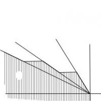 Description of production using technology set
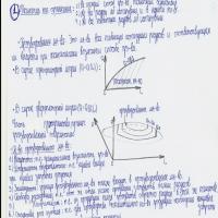 The concept of the production system and the production process
 Internet access using UserGate
 8 even channel distribution